Making Spatial Data from Plain Text

This tutorial is about using large language models to work with text as spatial data. A large language model (LLM) is a computational model designed to perform natural language processing tasks, especially language generation, using contextual relationships derived from a large set of training data (wikipedia). ChatGPT, and most other products that we refer to as "AI", are large language models.

In order to make spatial data from plain text, we need a bunch of text. This can take many forms, but for this tutorial I thought it would be interesting to work with data from StreetEasy. I wrote a python script to scrape rental listings in Manhattan, including their address, rent, and crucially their descriptions. These descriptions include qualitative descriptions of the properties that they are attached to. In this tutorial, we will use an LLM to turn those descriptions into data, in two different ways.

If you are interested in the scraping methodology, feel free to send an email and I can share those files.

The tutorial has two parts, both working from the same CSV of listings:

In Part 1, we use a language model to classify each listing description: does it primarily sell the neighborhood (location, transit, nearby amenities) or the unit itself (finishes, layout, appliances)? We aggregate those labels by census neighborhood and map the result as a choropleth.

In Part 2, we pass each description through an embedding model to get a high-dimensional vector that encodes its meaning. We then reduce those vectors down to 2D with UMAP, cluster them with k-means, auto-label each cluster, and map the results both geographically and semantically.

Environment setup

Working locally

Through most tutorials, you have used python notebooks in Google Colab. Colab is very convenient because it allows you to run code without having to worry about your local environment.

We won't use that for this tutorial, because we will be using a large language model locally. Meaning you will download the model, and run it locally on your own computer. Also, in the spirit of this class, while the service provided by Google is great, it's best if you learn how to use these tools and technologies in a way that doesn't leave you reliant on the services of one of the most powerful entities in the world.

All that said, if you are really struggling with setting up the environment, you can feel free to switch back to google colab. If you do that, you can skip the entire environment setup phase of this tutorial. You can stll run the model locally through the ollama app, or use an llm located somewhere else like ChatGPT. You'll need to edit the notebook a bit, mainly to import the created file back into this notebook as a geodataframe, let me know if you need assistance.

Setting up your notebook

So let's start. For this, you will need a full-featured text editor, I recommend vs code, and will assume you are using that in the following steps.

Let's open up terminal in MacOS, or Powershell in Windows. Run each of these commands by typing them into your terminal and hitting enter. Together they will create a folder name tutorial-12 on your desktop, open it, and create some (empty) files that we will need later. If you are new to this, I recommend this quick start on navigating your files in terminal. If this is all too confusing, you are absolutely welcome to create the folder as you would any other folder, open it in vs code, and create the files using the "new file" button in there.

In MacOS, run each of these one at a time by typing them into your terminal and hitting enter.

cd Desktop 
mkdir tutorial-12
cd tutorial-12
touch tutorial-12.ipynb
touch environment.yml
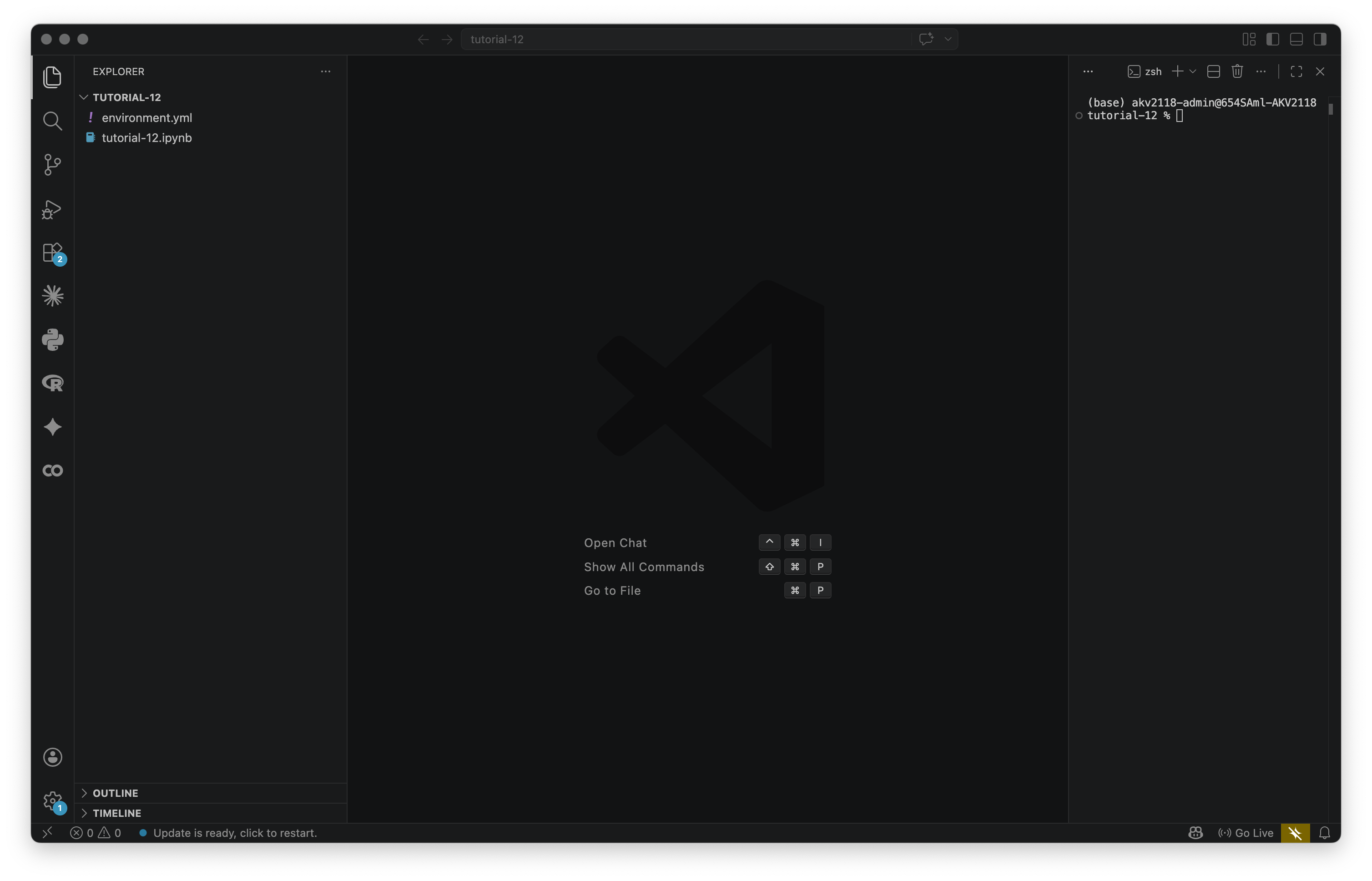
code .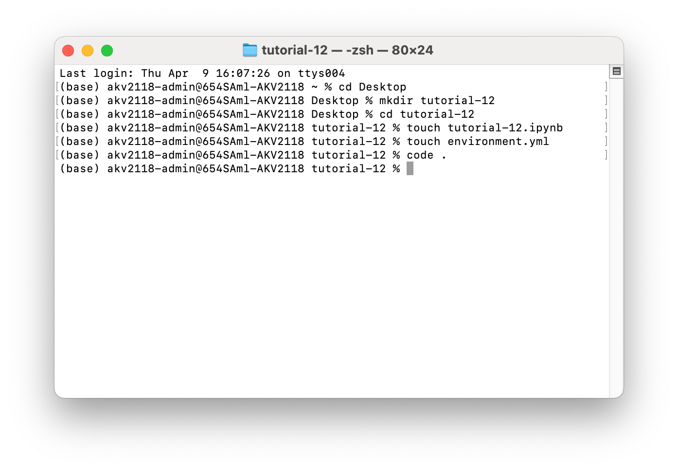

Most likely, that last command did not work for you. If it did, it would open vs code at the folder that you made, and you would see the files that you created on the "Explorer" tab on the left. If you would like to use that command, you can follow the instructions here. I personally find it convenient. If you prefer not to, you can open up VS code, and select your folder in File > Open Folder... If you are on windows, this command should work by default.

In Windows, open PowerShell and run:

cd Desktop
mkdir tutorial-12
cd tutorial-12
New-Item tutorial-12.ipynb
New-Item environment.yml
code .

One last thing: In VS Code, go to Terminal > New Terminal. This will open up a new terminal on the right side of your VS Code workspace, that is running in this folder. Going forward, this is where we will type terminal commands. You workspace should now look like the below.

Installing conda

In order to run this code, we will have to input various packages that are not included in vanilla python, such as geopandas, altair, etc. For various reasons, we will be using conda as a package manager, instead of the default python package manager, pip.

There are a few conda install options, we will choose Miniconda — it's the smallest version that gives you what you need. Download the Miniconda installer from anaconda.com/download and run it with all default settings.

On MacOS, after it finishes installing, run this to refresh your terminal session:

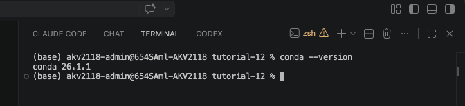
source ~/.zshrc

Then verify it worked:

conda --version

You should see a version number like the screenshot below. Once that works, you may proceed.

Creating the conda environment

We'll use an environment.yml file to set up the environment. You should have already created it, but if you haven't, do so now and paste the following into it:

name: tutorial-12
channels:
  - conda-forge
  - defaults
dependencies:
  - python
  - huggingface_hub
  - pandas
  - geopandas
  - numpy
  - scipy
  - umap-learn
  - scikit-learn
  - altair
  - plotly
  - ipykernel
  - nbformat
  - pip:
    - ollama
    - nbformat

conda-forge is listed first because it carries the most up-to-date geospatial builds. ipykernel is what lets you run the notebook in VS Code. ollama must be installed via pip (the python package manager,) hence why it looks different.

In your terminal run:

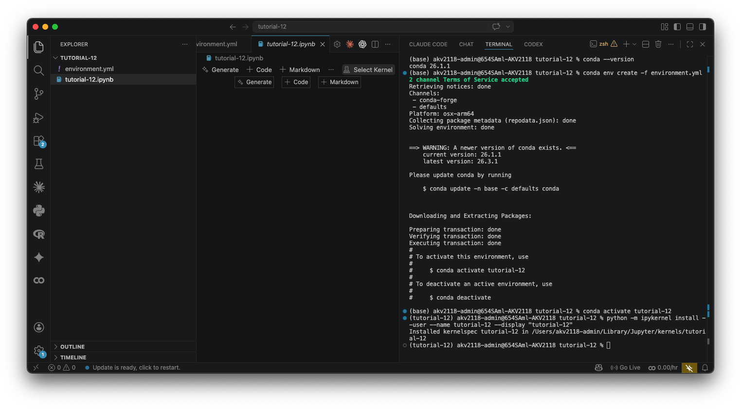
conda env create -f environment.yml

This will take a few minutes the first time. Once it's done:

conda activate tutorial-12

Your terminal prompt will change to show (tutorial-12). Then register the environment as a Jupyter kernel so VS Code can find it:

python -m ipykernel install --user --name tutorial-12 --display-name "tutorial-12"

You only need to do this once. After that, open the notebook (the .ipynb file) in VS Code, click the "Select Kernel" button in the top-right corner, click "Jupyter Kernel...", and choose tutorial-12. If you don't see it, close and reopen VS Code. Once the kernel is selected, we're all done with setup.

Setup

Like all technologies, all LLMs are built for a specific purpose. This notebook uses two different kinds of language models:

Part 1 uses a generation model — a model trained to generate something, in this case text. You ChatGPTs etc are general generation models (although increasingly these days they are stacks of multiple models.) We will use qwen3.5:2b, a very small, open-weight (not quite open-source) large language model developed by Alibaba. You can find the model card (information about the model) here. We are going to use this as a classifier by prompting it to read each listing and output a label.

Part 2 uses an embedding model — a model trained to produce vectors (in the machine learning sense) that encode meaning. If you don't know what that is, don't worry about it, I will explain a bit more when we get to that part. We will use nomic-embed-text, a completely open-source (meaning the training data is also open-sourced) embedding model developed by nomic.ai, which funnily enough looks like it is in the AEC business these days. You can find the model card here

While these models are different—you cannot use one in place of the other—they are similar in that they are both lightweight, and can easily run on any modern hardware. qwen3.5:2b is a 2 billion parameter model, tiny by LLM standards. nomic-embed-text is even smaller, with less than 200 million parameters. For a point of comparison, the highest quality models produced by labs like OpenAI and Anthropic are estimated to be 100 to 400 billion parameters.

We'll run both locally using Ollama. Ollama lets you download and run open-weight models on your own machine. Install it from ollama.ai, then pull the two models using the below commands. Note that you should have at least 4gb of free space on your computer before doing so:

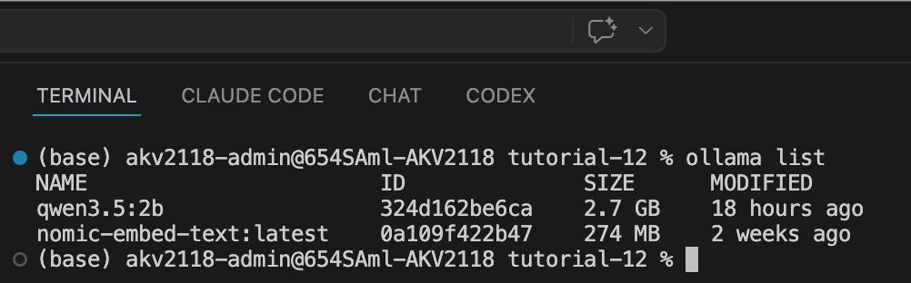
ollama pull qwen3.5:2b
ollama pull nomic-embed-text

After you pull those two, run ollama list, and it should look like the screenshot below.

Notice that these models are not small - this is about 3gb total of space. After you are finished with the tutorial, you are welcome to remove them using these commands:

ollama rm qwen3.5:2b
ollama rm nomic-embed-text

Alternative to Local LLMs

The tutorial will assume you are using a local LLM going forward. I think it is a good opportunity to see that this technology does not necessarily need data center level of computation. For many tasks, your computer is totally fine. But, if you prefer to use a cloud-based model, here are two options:

The simplest is just using a chatbot like ChatGPT or Claude directly — if you paste in the csv we are using and our prompt, it should do a good (if not better) job of classifying the descriptions.

Another option is HuggingFace. HuggingFace is a platform that hosts open-weight and open-source models — think of it like GitHub but for AI. When most people use an open source model, they use HuggingFace. They also offer an Inference API, which lets you send text to a model running on their servers and get a response back, without running anything locally. You'll need a free account and an API token from huggingface.co/settings/tokens, and then you would change the code below to make an API call to HuggingFace instead of Ollama.

The underlying logic is the same either way — you're writing a prompt and getting a response, the model just runs somewhere else.

Imports

Let's start by importing everything we'll need. Copy this into the first cell of your notebook and run it.

# Standard library
import os
import json
import time

# Data manipulation
import pandas as pd
import numpy as np

# Language model — Ollama (local)
import ollama

# Machine learning — used in Part 2
from sklearn.cluster import KMeans
from sklearn.preprocessing import normalize   # L2-normalizes vectors before clustering
from scipy.spatial.distance import cosine as cosine_distance
import umap
import nbformat

# Visualization — Altair for all maps and charts in both parts
import altair as alt
import plotly.express as px
alt.data_transformers.disable_max_rows()  # lift Altair's default 5000-row limit

# Geospatial — used in Part 1 for the NTA spatial join
import geopandas as gpd

print("Imports OK.")

It may take a minute. If you get an import error for any of these, make sure you've activated the tutorial-12 conda environment and selected it as the kernel in VS Code.

Load the dataset

Next, load the StreetEasy listings CSV and take a look at what we're working with. Create a new folder in your project called data/, and download the streeteasy_full.csv file here. In that folder is also a smaller csv (streeteasy_250,) If you would like to start with something that will run faster and scale up from there.

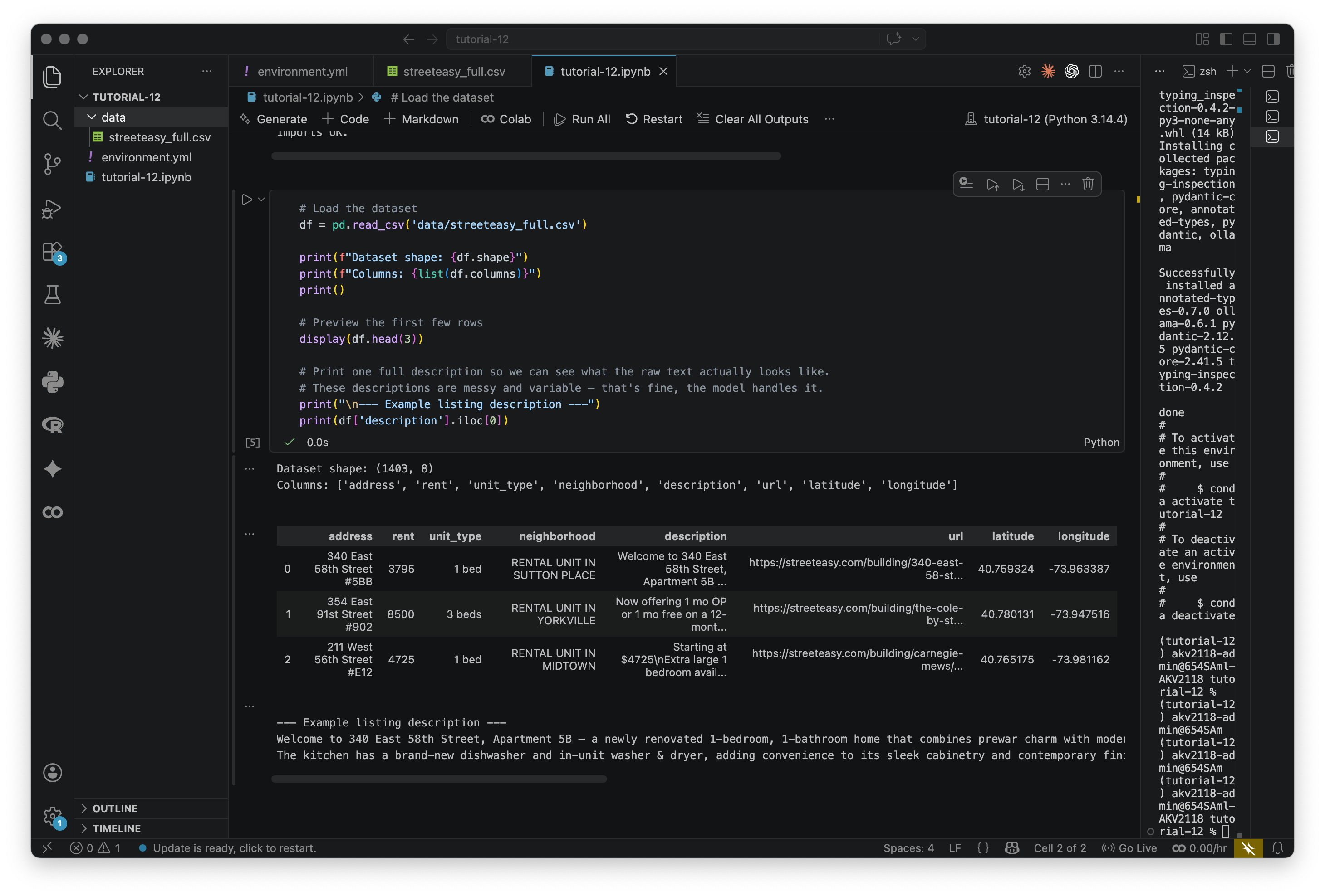
# Load the dataset
df = pd.read_csv('data/streeteasy_full.csv')

print(f"Dataset shape: {df.shape}")
print(f"Columns: {list(df.columns)}")
print()

# Preview the first few rows
display(df.head(3))

# Print one full description so we can see what the raw text actually looks like.
# These descriptions are messy and variable — that's fine, the model handles it.
print("\n--- Example listing description ---")
print(df['description'].iloc[0])

Take a look at the description that prints, it should look like below. These are real listings scraped from StreetEasy. Landlords are not known for their prose.

Part 1: Classification with Prompting

In this part we use the generation model to classify each listing description: does it primarily sell the neighborhood (transit, parks, character) or the unit itself (layout, finishes, light)?

We label each description 1 (neighborhood-forward) or 0 (unit-forward) using zero-shot prompting — no examples, no labeled training data, just a prompt. We then aggregate to the NTA (Neighborhood Tabulation Area) level and map the result as a choropleth.

Step 1.1: Define the generation model

First, let's define the model and make sure Ollama is running. We're using qwen3.5:2b. If you want to try something else, change GENERATION_MODEL to anything you've pulled with ollama pull, and swap out the model name. You can see a list of available models here. Keep in mind that some of these are likely way too large for your personal computer.

# ── Generation model setup ────────────────────────────────────────────────────
# Change this to switch models. Options:
#   'qwen3.5:2b'  — fast, good enough for binary classification
#   'qwen3.5:4b'  — more accurate, needs more RAM, slower
GENERATION_MODEL = 'qwen3.5:2b'

# Quick connectivity check — makes sure Ollama is running before the long loop.
try:
    _test = ollama.chat(
        model=GENERATION_MODEL,
        messages=[{'role': 'user', 'content': 'Reply with the word OK and nothing else.'}],
        think=False
    )
    print(f"Ollama OK — model: {GENERATION_MODEL}")
    print(f"Test response: {_test['message']['content'].strip()}")
except Exception as e:
    print(f"Could not reach Ollama: {e}")
    print("Make sure Ollama is running:")
    print(f"  ollama pull {GENERATION_MODEL}")
    print("  ollama serve   (if not already running as a background service)")

If this prints "Ollama OK" you're good. If not, Ollama probably isn't running — on Mac it should be visible in the menu bar, on other systems you may need to run ollama serve in a separate terminal.

Step 1.2: Classify each listing

Now we loop over every listing and ask the model to classify it. The function builds a prompt describing the two categories and asks for a single digit back — 1 for neighborhood-forward, 0 for unit-forward.

The prompt says "Reply with ONLY the digit 1 or 0" to make parsing easy. If a parse fails, it will assign -1, and exclude that listing from the dataset.

We also have included think=False in the code below. These days, most AI models for text generation are "reasoning" models. They perform an approximation of reasoning by prompting the model to think, which will cause the model to reprompt itself many times before answering your question. That can be a really powerful feature and leaving it on would probably yield better classifications, but for a relatively dumb one-shot classification task like this, it makes it far too slow.

Try reading a few descriptions yourself in the .csv before looking at what the model says. Where does it surprise you? Keep in mind this is a forced binary and highly imperfect — real listings are almost always going to be describing both the unit and the neighborhood.

This step takes 5-15 minutes for ~1400 listings, depending on your computer. Expect your computer to get a bit warm.

def classify_listing(description, model=GENERATION_MODEL):
    """
    Ask the LLM to classify a listing description.
    Returns 1 (neighborhood-forward), 0 (unit-forward), or -1 (parse failure).
    """
    prompt = (
        "You are classifying apartment rental listings.\n"
        "Read the listing description below and decide which it primarily emphasizes:\n\n"
        "  1 = NEIGHBORHOOD-FORWARD: mainly sells the location — "
        "transit, nearby parks, restaurants, walkability, neighborhood character.\n"
        "  0 = UNIT-FORWARD: mainly describes the apartment itself — "
        "finishes, layout, appliances, light, renovations.\n\n"
        "Reply with ONLY the digit 1 or 0. No explanation.\n\n"
        f"Listing:\n{description}"
    )
    response = ollama.chat(
        model=model,
        messages=[{'role': 'user', 'content': prompt}],
        think=False
    )
    raw = response['message']['content'].strip()
    if raw.startswith('1'):
        return 1
    elif raw.startswith('0'):
        return 0
    else:
        return -1  # model returned something unexpected — we'll drop these from the map


# ── Run classification ────────────────────────────────────────────────────────
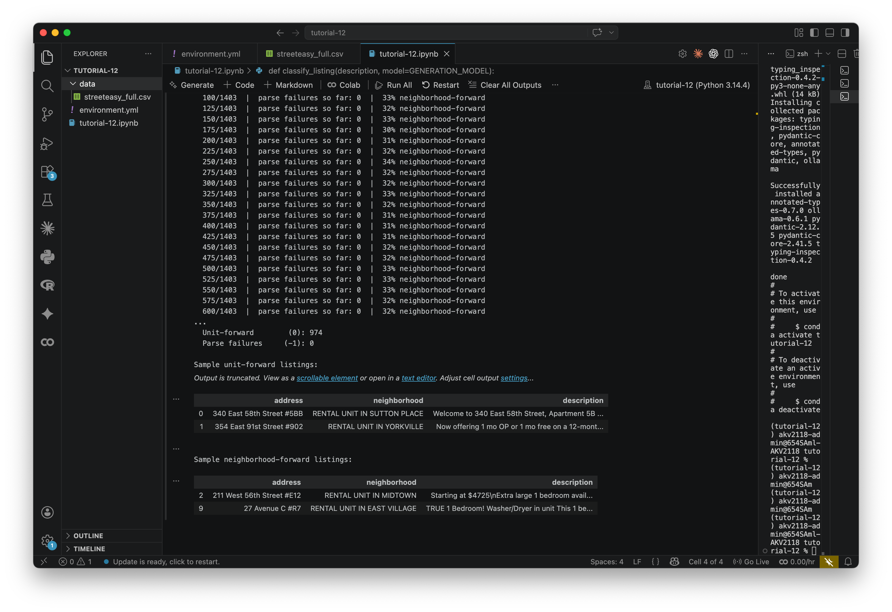
print(f"Classifying {len(df)} listings with {GENERATION_MODEL}...")

labels = []
for i, desc in enumerate(df['description']):
    label = classify_listing(str(desc))
    labels.append(label)
    if (i + 1) % 25 == 0:
        valid = [l for l in labels if l != -1]
        pct_nbhd = sum(valid) / len(valid) * 100 if valid else 0
        print(f"  {i + 1}/{len(df)}  |  parse failures so far: {labels.count(-1)}"
              f"  |  {pct_nbhd:.0f}% neighborhood-forward")

df['neighborhood_forward'] = labels

print(f"\nDone.")
print(f"  Neighborhood-forward (1): {labels.count(1)}")
print(f"  Unit-forward        (0): {labels.count(0)}")
print(f"  Parse failures     (-1): {labels.count(-1)}")

# Preview — look at a few disagreements to gut-check the model
print("\nSample unit-forward listings:")
display(df[df['neighborhood_forward'] == 0][['address', 'neighborhood', 'description']].head(2))
print("\nSample neighborhood-forward listings:")
display(df[df['neighborhood_forward'] == 1][['address', 'neighborhood', 'description']].head(2))

When it finishes, the bottom of your output should look like below. Take a look at the sample listings that print. Read the descriptions and see if you agree with the model's classification. It won't be perfect — this is a blunt instrument — but it should be directionally right where it is possible to be.

Step 1.3: Load Neighborhood Tabulation Areas

To map the results, we need a geographic boundary file. We'll use NYC's Neighborhood Tabulation Areas (NTAs) — the standard sub-borough census geography.

Before running this cell: download the NTA GeoJSON from NYC Open Data (export -> Geojson) and save it to your data/ folder, renamed to nta_nyc.geojson.

nta_gdf = gpd.read_file('data/nta_nyc.geojson')
print(f"Loaded {len(nta_gdf)} NTAs")
print(f"Columns: {list(nta_gdf.columns)}")

Now we do a spatial join. We filter to Manhattan NTAs, convert the listings to a GeoDataFrame, join each one to the NTA polygon it falls in, and compute the mean neighborhood_forward score per NTA.

This should feel familiar — we're doing the same thing here (joining points to polygons) as we did in Tutorial 1. Just with classification labels instead of tree counts.

# Filter to Manhattan and reproject to match the listings CRS
manhattan_nta = nta_gdf[nta_gdf['boroname'] == 'Manhattan'].copy()
manhattan_nta = manhattan_nta.to_crs('EPSG:4326')
print(f"Manhattan NTAs: {len(manhattan_nta)}")

# Drop parse failures (-1) before the spatial join
df_valid = df[df['neighborhood_forward'] != -1].copy()
print(f"Listings with valid classification: {len(df_valid)}")

# Convert listings to GeoDataFrame using their lat/lon coordinates
listings_gdf = gpd.GeoDataFrame(
    df_valid,
    geometry=gpd.points_from_xy(df_valid['longitude'], df_valid['latitude']),
    crs='EPSG:4326'
)

# Spatial join: assign each listing to the NTA polygon it falls within
joined = gpd.sjoin(
    listings_gdf,
    manhattan_nta[['ntaname', 'geometry']],
    how='left',
    predicate='within'
)

# Aggregate: mean neighborhood_forward per NTA
nta_scores = (
    joined.groupby('ntaname')['neighborhood_forward']
    .agg(avg_neighborhood_forward='mean', listing_count='count')
    .reset_index()
)

print(f"\nNTAs with at least one listing: {len(nta_scores)}")
print("\nTop 5 most neighborhood-forward:")
print(nta_scores.sort_values('avg_neighborhood_forward', ascending=False)
      .head(5)[['ntaname', 'avg_neighborhood_forward', 'listing_count']]
      .to_string(index=False))

Step 1.4: Map the result

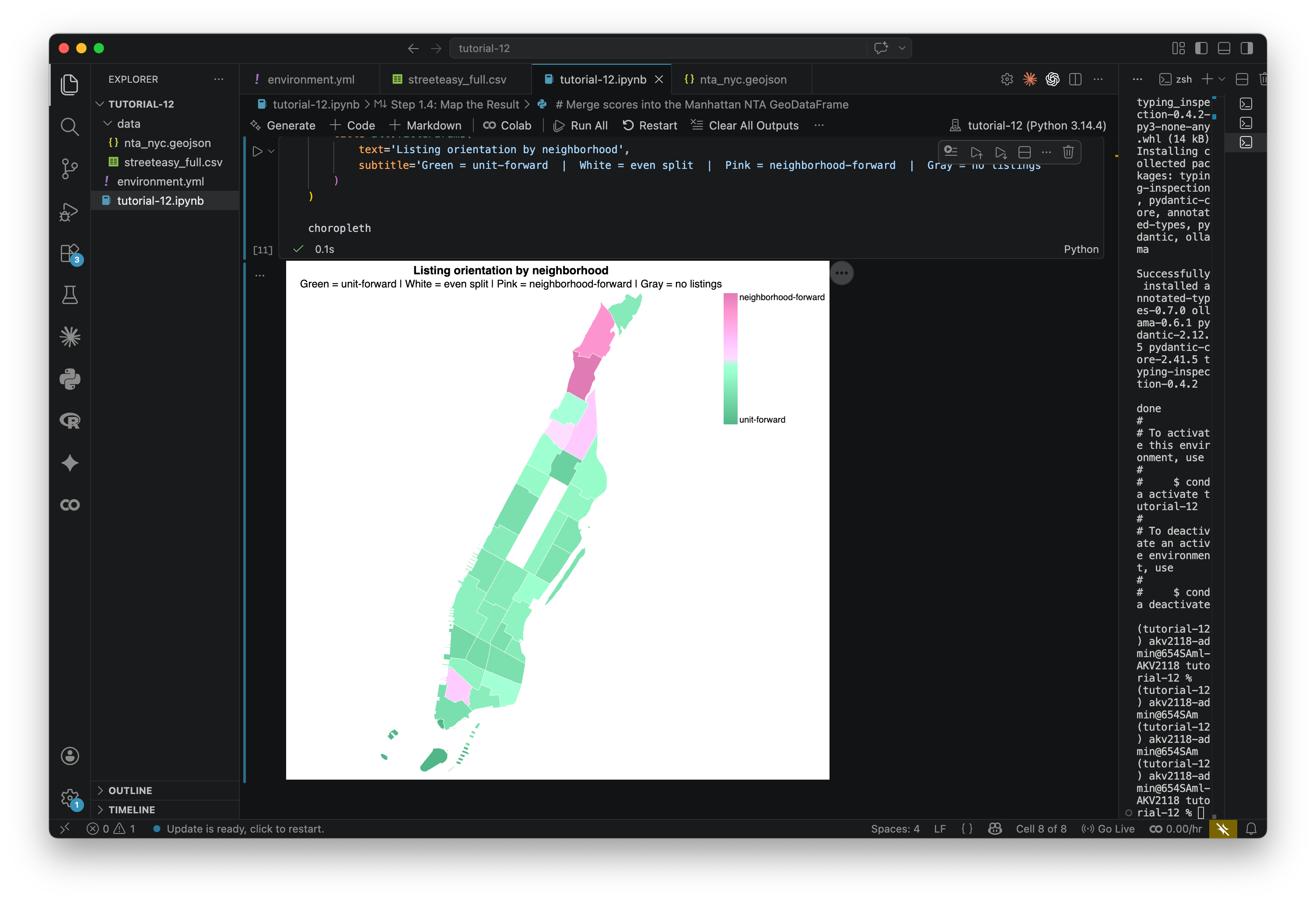
Now we'll build a choropleth of Manhattan NTAs. Each NTA is colored by its average neighborhood_forward score: pink means listings in that area tend to sell the location, green means they tend to sell the unit, white an even split.

# Merge scores into the Manhattan NTA GeoDataFrame
manhattan_scored = manhattan_nta.merge(nta_scores, on='ntaname', how='left')

# The NTA source file contains Timestamp columns that can't be JSON-serialized.
# Keep only the columns the chart actually needs.
cols_needed = ['ntaname', 'geometry', 'avg_neighborhood_forward', 'listing_count']
nta_geojson = json.loads(manhattan_scored[cols_needed].to_json())

choropleth = alt.Chart(
    alt.InlineData(values=nta_geojson, format=alt.DataFormat(property='features', type='json'))
).mark_geoshape(
    stroke='white',
    strokeWidth=0.5
).encode(
    color=alt.condition(
        'isValid(datum.properties.avg_neighborhood_forward)',
        alt.Color(
            'properties.avg_neighborhood_forward:Q',
            scale=alt.Scale(
                range=['#52b788', '#ffffff', '#e07bb5'],
                domain=[0, 0.5, 1]
            ),
            legend=alt.Legend(
                title='',
                values=[0, 1],
                labelExpr="datum.value === 0 ? 'unit-forward' : 'neighborhood-forward'",
                gradientLength=150
            )
        ),
        alt.value('#d0d0d0')
    ),
    tooltip=[
        alt.Tooltip('properties.ntaname:N', title='NTA'),
        alt.Tooltip('properties.avg_neighborhood_forward:Q', title='Avg score', format='.2f'),
        alt.Tooltip('properties.listing_count:Q', title='# listings in sample')
    ]
).project('mercator').properties(
    width=450, height=550,
    title=alt.TitleParams(
        text='Listing orientation by neighborhood',
        subtitle='Green = unit-forward  |  White = even split  |  Pink = neighborhood-forward  |  Gray = no listings'
    )
)

choropleth

Take a look at the result. Does the pattern make sense to you? To me, it doesn't totally make sense. I would guess that we are looking at the bias of our dataset: The description of listings probably talks about the unit mroe than the neighborhood. Still, there are some interesting outliers.

We can also export this scored NTA layer as a GeoJSON for use in other tools:

# Export scored NTA boundaries to GeoJSON
out_path = 'data/nta_scored.geojson'
manhattan_scored[cols_needed].to_file(out_path, driver='GeoJSON')
print(f"Saved → {out_path}")

from IPython.display import FileLink
FileLink(out_path, result_html_prefix="Download: ")

What prompts do you think would yield more interesting maps? That is what you will be asked to try in the assignment. If you are strapped for time, feel free to stop here and move to the assignment. However, if you can I do recommend continuing. I think part 2 is where things start to get interesting.

Part 2: Semantic Mapping with Embeddings

In Part 1 we gave the model instructions and asked for a label. In Part 2 we do something different — we turn each description into a vector of numbers, and use those vectors to build a map of meaning rather than geography.

What are embeddings?

When a language model is trained, it learns to represent words and phrases as lists of numbers called vectors (or embeddings). Things with similar meanings end up with similar numbers. "Steps from the park" and "across from the park entrance" will have nearly identical vectors even though they share no words, because the model learned that both describe similar things.

We apply that at the scale of whole listing descriptions. Each description gets compressed into a single vector — 768 numbers, for the model we're using. That vector is a coordinate in a 768-dimensional space, where closeness means similarity of meaning.

This same idea shows up in a lot of places we've talked about in this course. AlphaEarth does it for satellite imagery — every pixel gets a vector, and the result is a space where similar land cover types cluster together regardless of geography. The targeting systems we discussed in The Curse of Dimensionality work the same way: people, places, and behaviors get converted to vectors, and "similarity to a target profile" is just a distance calculation. When you type a message to ChatGPT, every word is immediately converted to an embedding before any processing happens. The model works entirely in this numerical space. Embeddings are the substrate of how these models operate.

Step 2.1: Generate embeddings

We pass each description through the embedding model, which converts it to a vector. This runs locally through Ollama, same as before. We're using nomic-embed-text, which produces 768-dimensional vectors. If you're curious how it compares to other options, the MTEB leaderboard is the standard benchmark — look at the "Semantic Textual Similarity" column. If you want something stronger and have the RAM, try mxbai-embed-large (ollama pull mxbai-embed-large). Just note that embeddings from different models aren't interchangeable — you can't mix vectors from two models and compare them.

This step takes 1-5 minutes for ~1400 listings

# Load the dataset (allows this cell to run independently of Part 1)
df = pd.read_csv('data/streeteasy_full.csv')

# Calls Ollama running on your machine. Requires: ollama pull nomic-embed-text
# Produces 768-dimensional vectors.
def embed_local(text):
    response = ollama.embeddings(model='nomic-embed-text', prompt=text)
    return response['embedding']

embed = embed_local


# ---- Run embeddings ------------------------------------------------
print(f"Generating embeddings for {len(df)} listings...")
print("(Expect ~1-5 minutes on a laptop.)")
print()

embeddings = []
for i, text in enumerate(df['description']):
    # str() guards against NaN values in the description column
    embeddings.append(embed(str(text)))
    # Print progress every 50 rows
    if (i + 1) % 50 == 0:
        print(f"  {i + 1} / {len(df)} listings processed...")

df['embedding'] = embeddings

print(f"\nDone. Each embedding has {len(df['embedding'].iloc[0])} dimensions.")

Once that runs, each listing has a 768-number vector attached to it. To get a feel for what these capture, let's compare a few pairs:

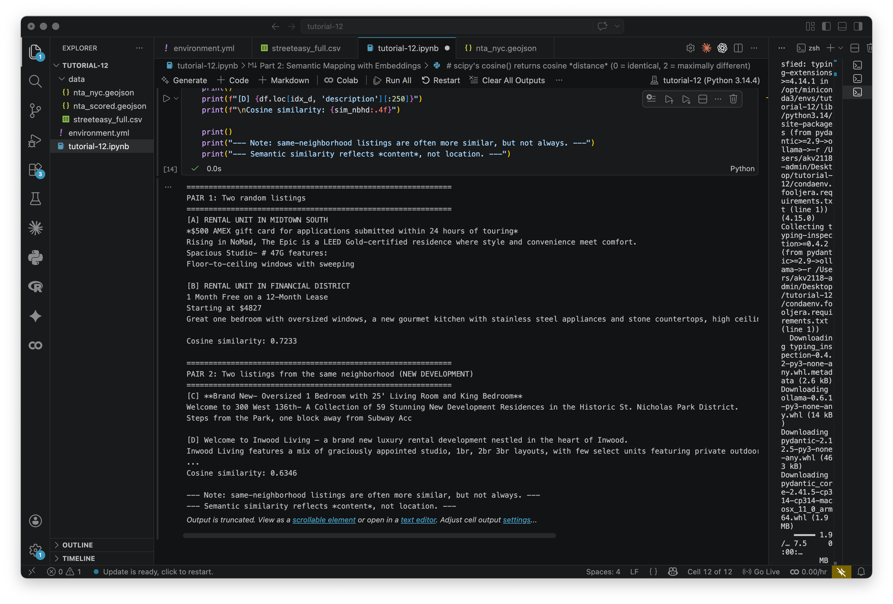
# scipy's cosine() returns cosine *distance* (0 = identical, 2 = maximally different)
# We convert to similarity by subtracting from 1, so: 1 = identical, -1 = opposite
def cosine_sim(a, b):
    return 1 - cosine_distance(a, b)


# --- Pair 1: two randomly chosen listings ---
random_pair = df.sample(2, random_state=7)
idx_a, idx_b = random_pair.index.tolist()

sim_random = cosine_sim(df.loc[idx_a, 'embedding'], df.loc[idx_b, 'embedding'])

print("=" * 60)
print("PAIR 1: Two random listings")
print("=" * 60)
print(f"[A] {df.loc[idx_a, 'neighborhood']}")
print(df.loc[idx_a, 'description'][:250])
print()
print(f"[B] {df.loc[idx_b, 'neighborhood']}")
print(df.loc[idx_b, 'description'][:250])
print(f"\nCosine similarity: {sim_random:.4f}")


# --- Pair 2: two listings from the same neighborhood ---
same_nbhd_name = df['neighborhood'].value_counts().idxmax()
nbhd_pair = df[df['neighborhood'] == same_nbhd_name].sample(2, random_state=42)
idx_c, idx_d = nbhd_pair.index.tolist()

sim_nbhd = cosine_sim(df.loc[idx_c, 'embedding'], df.loc[idx_d, 'embedding'])

print()
print("=" * 60)
print(f"PAIR 2: Two listings from the same neighborhood ({same_nbhd_name})")
print("=" * 60)
print(f"[C] {df.loc[idx_c, 'description'][:250]}")
print()
print(f"[D] {df.loc[idx_d, 'description'][:250]}")
print(f"\nCosine similarity: {sim_nbhd:.4f}")

print()
print("--- Note: same-neighborhood listings are often more similar, but not always. ---")
print("--- Semantic similarity reflects *content*, not location. ---")

Read the descriptions and look at the scores. Listings from the same neighborhood are often similar, but not always — similarity here reflects what the description says, not where the apartment is.

Step 2.2: Dimensionality reduction with UMAP

768 dimensions can't be visualized, so we need to compress them. UMAP (Uniform Manifold Approximation and Projection) takes high-dimensional data and projects it to 2D (or 3D) while trying to keep nearby things nearby.

The result is a kind of semantic map. Two listings that describe similar things will land close together even if they share no words and are in different neighborhoods. The axes don't mean anything geographically — only the distances between points matter.

# Stack all embedding vectors into a 2D numpy array: shape = (n_listings, n_dimensions)
embedding_matrix = np.array(df['embedding'].tolist())
print(f"Embedding matrix shape: {embedding_matrix.shape}")

# 2D UMAP — used for the scatter plots and geographic comparison
reducer_2d = umap.UMAP(n_neighbors=15, min_dist=0.1, n_components=2, random_state=42)
umap_2d = reducer_2d.fit_transform(embedding_matrix)
df['umap_x'] = umap_2d[:, 0]
df['umap_y'] = umap_2d[:, 1]

# 3D UMAP — used for interactive 3D exploration after clustering
reducer_3d = umap.UMAP(n_neighbors=15, min_dist=0.1, n_components=3, random_state=42)
umap_3d = reducer_3d.fit_transform(embedding_matrix)
df['umap_x3'] = umap_3d[:, 0]
df['umap_y3'] = umap_3d[:, 1]
df['umap_z3'] = umap_3d[:, 2]

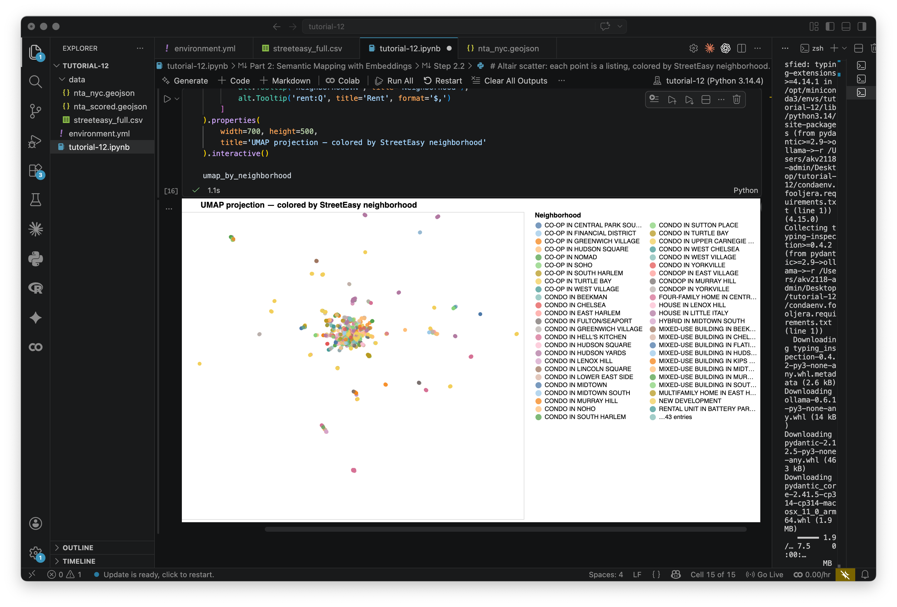
print("UMAP complete (2D and 3D).")

Now let's plot the 2D projection, with each point colored by its StreetEasy neighborhood:

# Altair scatter: each point is a listing, colored by StreetEasy neighborhood.
# Hover over any point to see the address, neighborhood, and rent.
# Use scroll to zoom, click-drag to pan.

umap_by_neighborhood = alt.Chart(df).mark_circle(size=40, opacity=0.75).encode(
    x=alt.X('umap_x:Q', axis=None, title=None),
    y=alt.Y('umap_y:Q', axis=None, title=None),
    color=alt.Color(
        'neighborhood:N',
        scale=alt.Scale(scheme='tableau20'),
        legend=alt.Legend(title='Neighborhood', columns=2, symbolLimit=50)
    ),
    tooltip=[
        alt.Tooltip('address:N', title='Address'),
        alt.Tooltip('neighborhood:N', title='Neighborhood'),
        alt.Tooltip('rent:Q', title='Rent', format='$,')
    ]
).properties(
    width=700, height=500,
    title='UMAP projection — colored by StreetEasy neighborhood'
).interactive()

umap_by_neighborhood

This is interactive, hover over the points. Notice how listings from the same neighborhood often cluster together — but not always. Some clusters cut across neighborhood lines, grouping by description style rather than location. This map shows similarity of language, not similarity of geography.

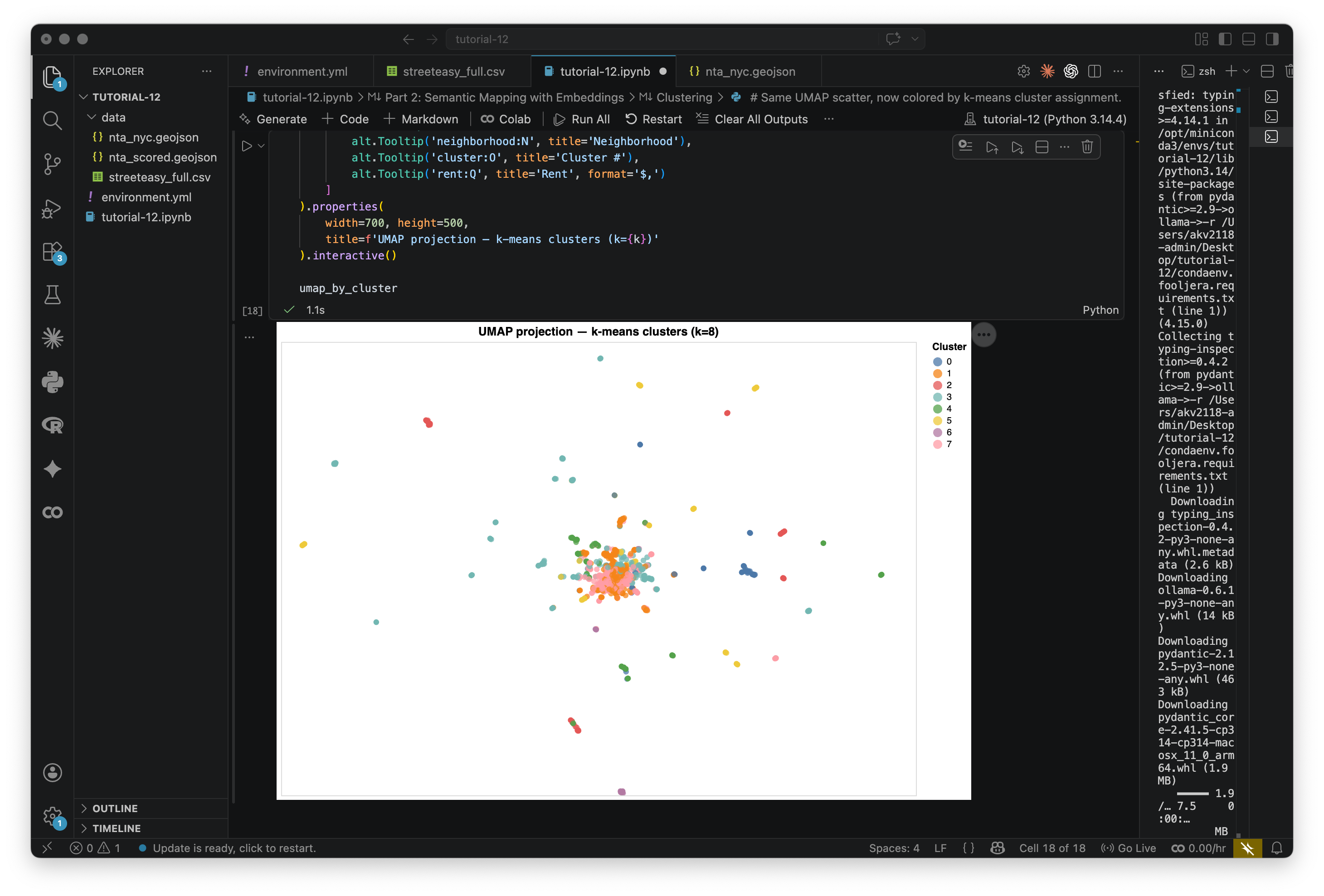
Step 2.3: Clustering

Now we use k-means clustering to group the listings into k clusters based on their position in embedding space. K-means works by repeatedly assigning each point to its nearest cluster center, then moving the center to the mean of its members, until stable.

Unlike Part 1, where we told the model what categories to use, here we're letting groupings emerge from the data. Try changing k between 5 and 12 and see what shifts. We cluster in the original high-dimensional space rather than the UMAP 2D, because UMAP compresses information and clustering there gives noisier results.

# Try changing k between 5 and 12 to see how the clusters shift
k = 8

# L2-normalize the embedding vectors before clustering.
# This makes k-means use cosine similarity rather than Euclidean distance,
# which is more appropriate for text embeddings (we care about direction, not magnitude).
embedding_matrix_normalized = normalize(embedding_matrix, norm='l2')

# Fit k-means on the full high-dimensional normalized embeddings
kmeans = KMeans(n_clusters=k, random_state=42, n_init=10)
df['cluster'] = kmeans.fit_predict(embedding_matrix_normalized)

print(f"K-means complete (k={k}).")
print()
print("Listings per cluster:")
print(df['cluster'].value_counts().sort_index())

Let's visualize the clusters on the UMAP scatter:

# Same UMAP scatter, now colored by k-means cluster assignment.

umap_by_cluster = alt.Chart(df).mark_circle(size=40, opacity=0.75).encode(
    x=alt.X('umap_x:Q', axis=None, title=None),
    y=alt.Y('umap_y:Q', axis=None, title=None),
    color=alt.Color(
        'cluster:O',
        scale=alt.Scale(scheme='tableau10'),
        legend=alt.Legend(title='Cluster')
    ),
    tooltip=[
        alt.Tooltip('address:N', title='Address'),
        alt.Tooltip('neighborhood:N', title='Neighborhood'),
        alt.Tooltip('cluster:O', title='Cluster #'),
        alt.Tooltip('rent:Q', title='Rent', format='$,')
    ]
).properties(
    width=700, height=500,
    title=f'UMAP projection — k-means clusters (k={k})'
).interactive()

umap_by_cluster

Below is what I get with eight clusters:

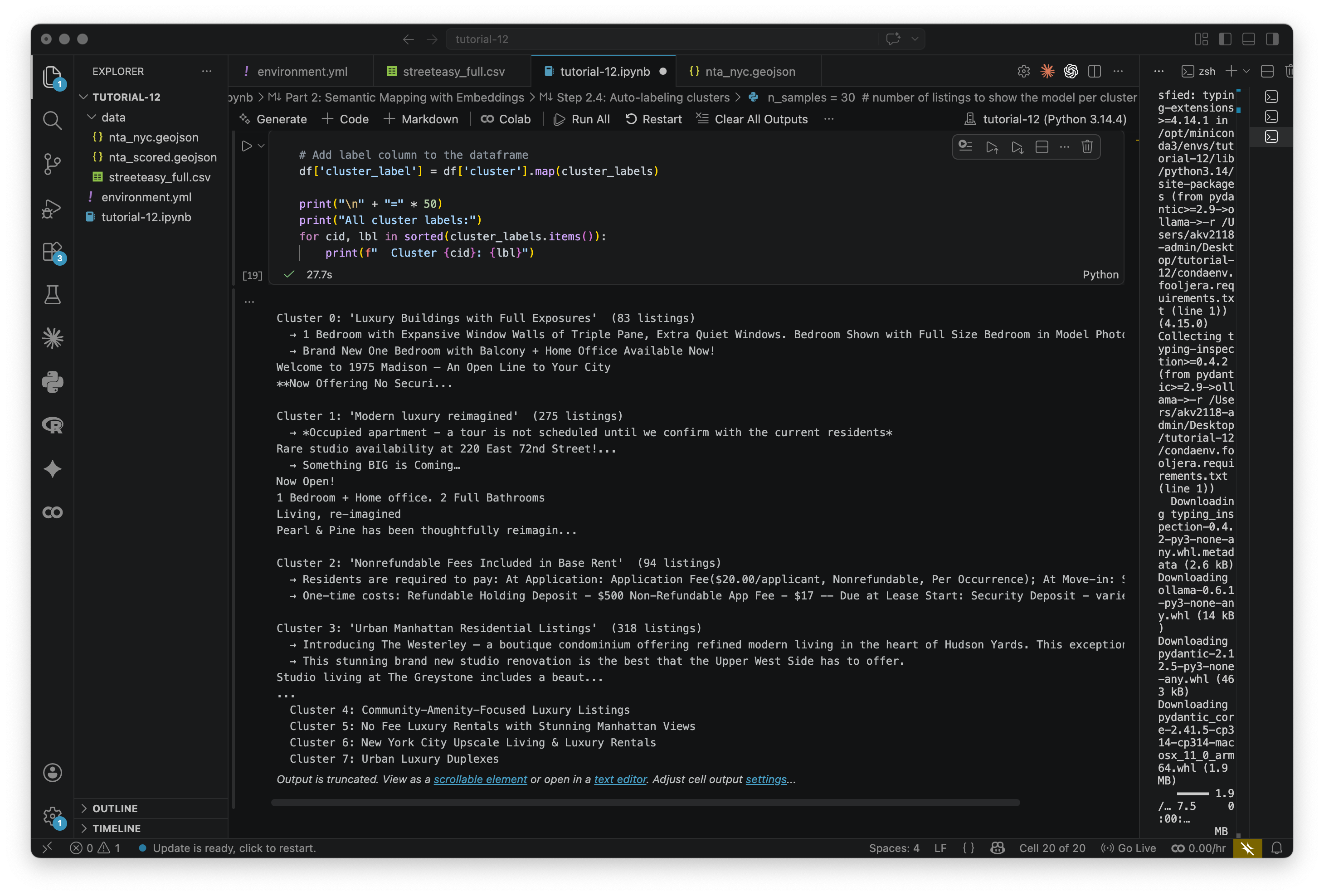
Step 2.4: Auto-labeling clusters

Each cluster has a number but no name. What is good at analyzing text? That's right, the generation model that we used before. We'll pass a sample of listings from each cluster to the generation model and ask it to describe what they have in common.

Here, the model is reading a group and naming a pattern, not making a judgment about a single item. This should be quicker than the last time we used this model, but that may increase if you change n_samples or the prompt.

n_samples = 30  # number of listings to show the model per cluster

cluster_labels = {}  # will hold { cluster_id: label_string }

for cluster_id in sorted(df['cluster'].unique()):
    # Get all listings in this cluster
    cluster_df = df[df['cluster'] == cluster_id]

    # Sample up to n_samples listings (use all if the cluster is small)
    sample_texts = cluster_df['description'].sample(
        min(n_samples, len(cluster_df)), random_state=42
    ).tolist()

    # Build a list of truncated descriptions for the prompt
    descriptions_block = "\n\n".join(
        [f"- {text[:300]}" for text in sample_texts]
    )

    # Ask what DISTINGUISHES this cluster, not what all listings share in general.
    prompt = (
        "You are labeling clusters in a semantic analysis of Manhattan apartment listing descriptions.\n\n"
        "The listings below were grouped together because they share a distinctive marketing angle or writing style. "
        "In 3–5 words, label what makes THIS cluster distinctive from other listings — "
        "what do these descriptions emphasize or lead with?\n\n"
        "Do NOT use the words 'apartment', 'rental', or 'unit'.\n"
        "Do NOT copy URLs, phone numbers, or contact details from the text.\n"
        "Return ONLY the label. No explanation.\n\n"
        f"Listings:\n{descriptions_block}"
    )

    response = ollama.chat(
        model=GENERATION_MODEL,
        messages=[{'role': 'user', 'content': prompt}],
        think=False
    )
    label = response['message']['content'].strip()

    cluster_labels[cluster_id] = label

    # Print a summary so we can sanity-check the label
    print(f"\nCluster {cluster_id}: '{label}'  ({len(cluster_df)} listings)")
    for ex in sample_texts[:2]:
        print(f"  → {ex[:140]}...")

# Add label column to the dataframe
df['cluster_label'] = df['cluster'].map(cluster_labels)

print("\n" + "=" * 50)
print("All cluster labels:")
for cid, lbl in sorted(cluster_labels.items()):
    print(f"  Cluster {cid}: {lbl}")

Read through the labels and the sample listings. Do they make sense? I find it not surprising that the most descriptions have the word luxury in there somewhere. Sometimes the model is too generic or too specific — re-run the cell or tweak the prompt if you want to push it in a different direction.

Step 2.5: Map the results

Now we map everything. Same listings, two views: a geographic map with listings at their real lat/lon, and a 3D semantic map with listings in UMAP space. Both colored by cluster. I recommend pasting each of the three scripts below as seperate cells, and then running them together. The third one will be a side-by-side visualization.

Where do geographic neighbors end up in different clusters? Any interesting trends you are noticing?

First, the geographic map:

# Filter out geocoding errors (coordinates outside Manhattan)
_in_manhattan = (
    (df['latitude']  >= 40.70) & (df['latitude']  <= 40.88) &
    (df['longitude'] >= -74.02) & (df['longitude'] <= -73.91)
)
df_geo = df[_in_manhattan].copy()
print(f"Using {len(df_geo)} of {len(df)} listings ({len(df) - len(df_geo)} excluded as geocoding errors)")

# Pre-compute a color map so all three figures use identical colors for each cluster label.
_T10 = px.colors.qualitative.T10
_clusters = sorted(df['cluster_label'].unique())
_color_map = {c: _T10[i % len(_T10)] for i, c in enumerate(_clusters)}

# Geographic map: listings at real lat/lon on a monotone tile basemap
geo_fig = px.scatter_mapbox(
    df_geo,
    lat='latitude',
    lon='longitude',
    color='cluster_label',
    color_discrete_map=_color_map,
    hover_name='address',
    hover_data={'neighborhood': True, 'rent': ':$,.0f', 'latitude': False, 'longitude': False},
    opacity=0.8,
    zoom=10.5,
    center={'lat': 40.775, 'lon': -73.97},
    title='Geographic map',
)
geo_fig.update_traces(marker=dict(size=7))
geo_fig.update_layout(
    mapbox_style='carto-positron',
    legend=dict(title='Cluster'),
    margin=dict(l=0, r=0, b=0, t=40),
    height=550,
)
geo_fig.show()

Now the 3D semantic map. This is interactive — drag to rotate, scroll to zoom, hover for details.

sem_fig = px.scatter_3d(
    df,
    x='umap_x3', y='umap_y3', z='umap_z3',
    color='cluster_label',
    color_discrete_map=_color_map,
    hover_name='address',
    hover_data={
        'neighborhood': True,
        'rent': ':$,.0f',
        'umap_x3': False,
        'umap_y3': False,
        'umap_z3': False,
    },
    opacity=0.8,
    title='3D Semantic Map',
)
sem_fig.update_traces(marker=dict(size=3))
sem_fig.update_layout(
    legend=dict(title='Cluster'),
    scene=dict(
        xaxis=dict(showticklabels=False, title=''),
        yaxis=dict(showticklabels=False, title=''),
        zaxis=dict(showticklabels=False, title=''),
    ),
    margin=dict(l=0, r=0, b=0, t=40),
    height=550,
)
sem_fig.show()

And finally, both side by side:

from plotly.subplots import make_subplots
import plotly.graph_objects as go

fig_combined = make_subplots(
    rows=1, cols=2,
    specs=[[{'type': 'map'}, {'type': 'scene'}]],
    subplot_titles=['Geographic map', 'Semantic map'],
    column_widths=[0.5, 0.5],
)

for cluster in _clusters:
    color = _color_map[cluster]
    geo_sub = df_geo[df_geo['cluster_label'] == cluster]
    sem_sub = df[df['cluster_label'] == cluster]

    fig_combined.add_trace(
        go.Scattermap(
            lat=geo_sub['latitude'],
            lon=geo_sub['longitude'],
            mode='markers',
            marker=dict(size=7, color=color),
            name=cluster,
            legendgroup=cluster,
            text=geo_sub['address'],
            customdata=geo_sub[['neighborhood', 'rent']].values,
            hovertemplate='<b>%{text}</b><br>%{customdata[0]}<br>$%{customdata[1]:,.0f}<extra></extra>',
        ),
        row=1, col=1,
    )

    fig_combined.add_trace(
        go.Scatter3d(
            x=sem_sub['umap_x3'],
            y=sem_sub['umap_y3'],
            z=sem_sub['umap_z3'],
            mode='markers',
            marker=dict(size=3, color=color, opacity=0.8),
            name=cluster,
            legendgroup=cluster,
            showlegend=False,
            text=sem_sub['address'],
            customdata=sem_sub[['neighborhood']].values,
            hovertemplate='<b>%{text}</b><br>%{customdata[0]}<extra></extra>',
        ),
        row=1, col=2,
    )

fig_combined.update_layout(
    map=dict(
        style='carto-positron',
        center=dict(lat=40.775, lon=-73.97),
        zoom=10.5,
    ),
    scene=dict(
        xaxis=dict(showticklabels=False, title=''),
        yaxis=dict(showticklabels=False, title=''),
        zaxis=dict(showticklabels=False, title=''),
    ),
    height=600,
    legend=dict(title='Cluster'),
    title=dict(
        text='Geographic vs. Semantic',
        x=0.5,
        xanchor='center',
    ),
    margin=dict(t=60, l=0, r=0, b=0),
)

fig_combined.show()

The output should look like the below, the map and embedding space side by side.

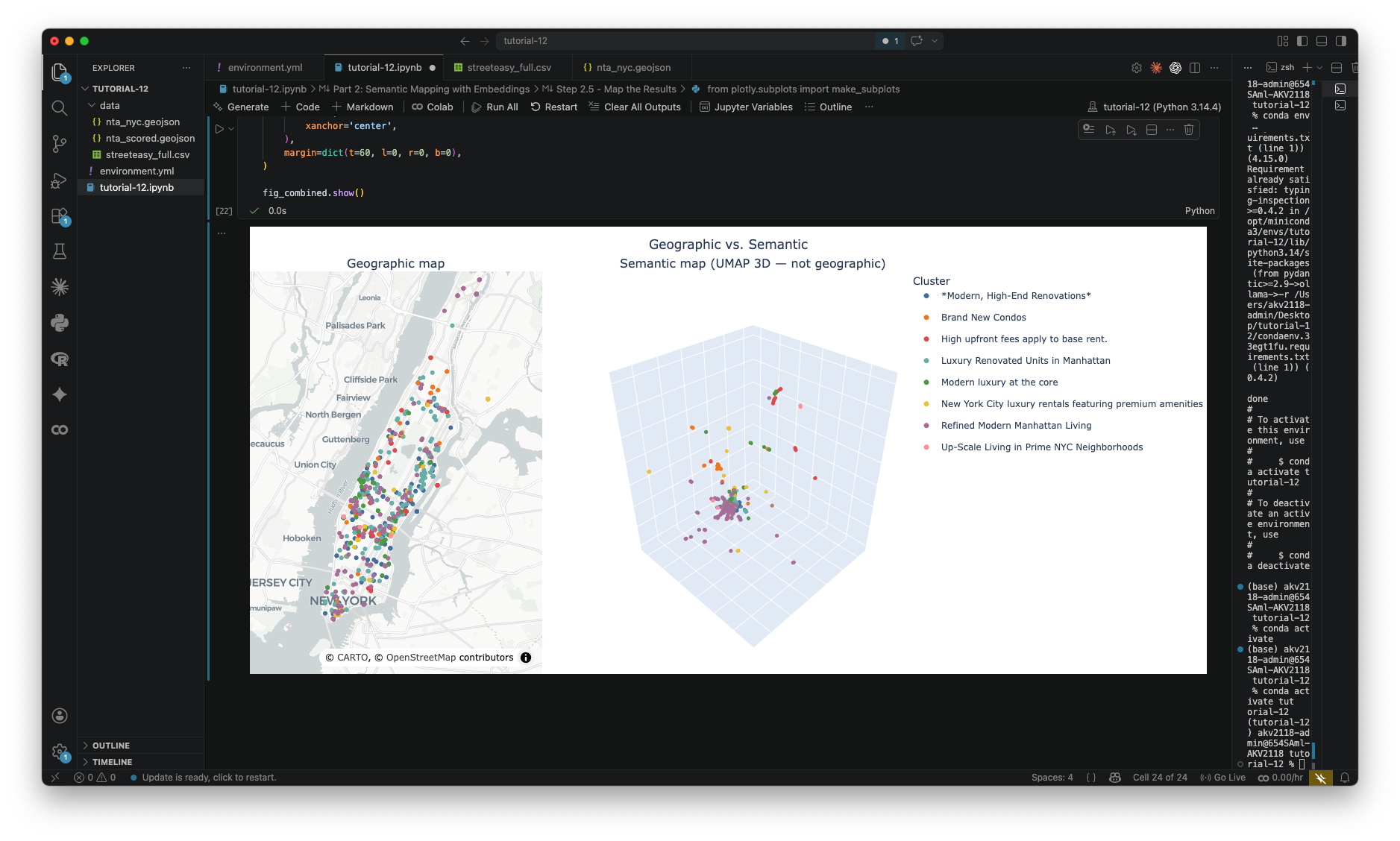
Spend some time with this. Rotate the semantic map and hover over points. Find two listings that are geographically close but in different clusters, and read their descriptions. Find two that are far apart geographically but in the same cluster. What is it about the language that connects or separates them?

While the assignment does not ask you to construct embeddings, if anyone ends up with any interesting results, I would love to see them!

Module by Adam Vosburgh, Spring 2026.